-
Gallery of Images:

-
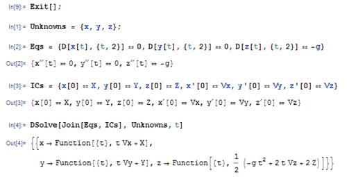
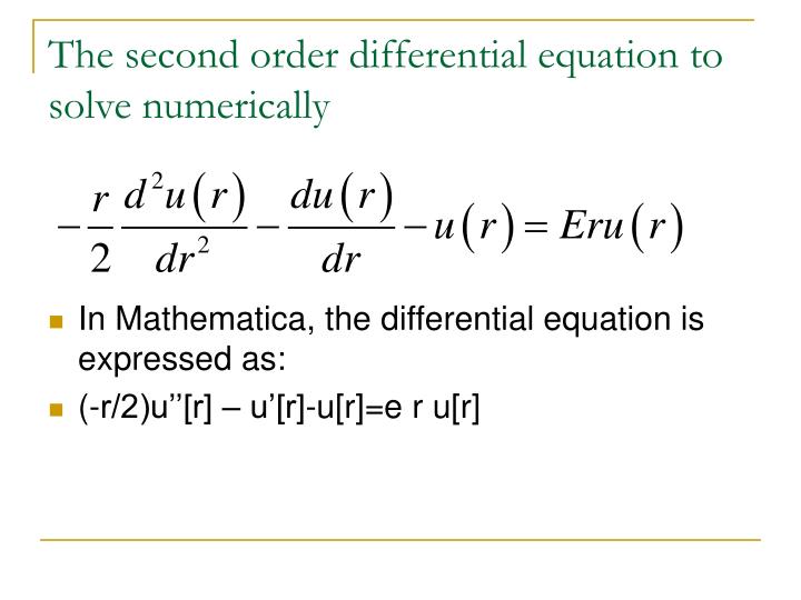
Get an overview of Mathematica's framework for solving differential equations in this presentation from Mathematica Experts Live: Numeric Modeling in Mathema Here is a set of notes used by Paul Dawkins to teach his Differential Equations course at Lamar University. Included are most of the standard topics in 1st and 2nd order differential equations, Laplace transforms, systems of differential eqauations, series solutions as well as a brief introduction to boundary value problems, Fourier series and partial differntial equations. Solving a matrix differential equation with Mathematica. Solving systems of second order differential equations. Solving a differential equation in Mathematica. Solving nonlinear system of differential equations in wolfram mathematica. Hot Network Questions The 3rd variation of the Differential Equations with Mathematica integrates new purposes from a number of fields, especially biology, physics, and engineering. the hot guide is additionally thoroughly suitable with contemporary models of Mathematica and is an ideal advent for Mathematica newbies. How to solve differential equations in Mathematica. Solving First Order and Second Order Differential equations Solving Differential Equations with boundary. In mathematics, an ordinary differential equation (ODE) Among ordinary differential equations, linear differential equations play a prominent role for several reasons. Mathematica, a proprietary application primarily intended for symbolic calculations. You can use the Wolfram Language function DSolve to find symbolic solutions to ordinary and partial differential equations. Solving a differential equation consists essentially in finding the form of an unknown function. Enterprise Mathematica; WolframAlpha Appliance. DSolve is set up to handle not only ordinary differential equations. Partial Differential Equations. Version 11 adds extensive support for symbolic solutions of boundary value problems related to classical and modern PDEs. Numerical PDEsolving capabilities have been enhanced to include events, sensitivity computation, new types of boundary conditions, and better complexvalued PDE solutions. Wolfram Community forum discussion about Using Mathematica in Teaching Differential Equations. Stay on top of important topics and build connections by joining. Mathematica provides friendly tools to solve and plot solutions to differential equations, but it is certainly not a panacea of all problems. This computer algebra system has tremendous plotting capabilities. The purpose of this book is to provide a traditional treatment of elementary ordinary differential equations while introducing the computerassisted methods that are now available with Mathematica. We have chosen Mathematica over other systems of computer algebra because of its combination of easy access and computational power, as evidenced through symbolic, numerical, and graphical output. The Wolfram Language ' s differential equation solving functions can be applied to many different classes of differential equations, automatically selecting the appropriate algorithms without needing preprocessing by the user. I have the next figure with inflow and outflow rates: And I need to calculate the time for which the pollution will be 50 from the initial value. Assuming that all lakes have the same pollution Here are my online notes for my differential equations course that I teach here at Lamar University. Despite the fact that these are my class notes, they should be accessible to anyone This is a preliminary version of the book Ordinary Differential Equations and Dynamical Systems. Mathematica, can help with the investigation of dierential equations. However, the course is not tied to Mathematica and any similar program can be used as well. Updates Tuitorial 2: Differential equations in Mathematica: Analytic solutions Brian Washburn, Version 1. 0, Off@General: : spellD; Differential equations solved analytically in Mathematica Typically one uses the function DSolve? DSolve a differential equation for the function y, with independent variable Goals and Emphasis of the Book Mathematicians have begun to find productive ways to incorporate computing power into the mathematics curriculum. There is no attempt here to use computing to avoid doing differential equations and linear algebra. The goal is to make some first ex plorations in the subject accessible to students who have had one year of calculus. Solve Differential Equation Solve a differential equation analytically by using the dsolve function, with or without initial conditions. To solve a system of differential equations, see Solve a. Buy Differential Equations with Mathematica on Amazon. com FREE SHIPPING on qualified orders Mathematica The# 1 tool for creating Demonstrations and anything technical. WolframAlpha Explore anything with the first computational knowledge engine. Differential Equations with Mathematica 3e is a supplemental text that can enrich and enhance any first course in ordinary differential equations. Designed to accompany Wileys ODE texts written by BrannanBoyce, BoyceDiPrima, BorrelliColeman and LomenLovelock, this supplement helps instructors move towards an earlier use of numerical and geometric methods, place a greater. Preface What follows are my lecture notes for a rst course in differential equations, taught at the Hong Kong University of Science and Technology. Differential Equations with Mathematica, Fourth Edition is a supplementing reference which uses the fundamental concepts of the popular platform to solve (analytically, numerically, andor graphically) differential equations of interest to students, instructors, and scientists. UHoensch Differential Equations and Applications Using Mathematica. pdf Ebook download as PDF File (. Solve a system of differential equations by specifying the equations as a vector. dsolve returns a structure containing the solutions. Solve the system of equations Early training in the elementary techniques of partial differential equations is invaluable to students in engineering and the sciences as well as mathematics. However, to be effective, an undergraduate introduction must be carefully designed to be challenging, yet still reasonable in its demands. Differential Equations with Mathematica, Fourth Edition is a supplementing reference which uses the fundamental concepts of the popular platform to solve (analytically, numerically, andor graphically) differential equations of interest to students, instructors, and scientists. University of Ioannina, Greece University of Rozousse, Bulgaria NEW JERSEY 6 LONDON SINGAPORE BElJlNG SHANGHAI HONG KONG TAIPEI CHENNAI Ioannis P Stavroulakis Stepan A Tersian PARTIAL DIFFERENTIAL EQUATIONS (Scond Edition) An Introduction with Mathematica This report gives the result of running a number of partial differential equations in Mathematica and Maple. The following systems were used at this time. Find differential equations satisfied by a given function: differential equations sin 2x. differential equations J2(x) More examples. Numerical Differential Equation Solving Numerically solve a differential equation using a variety of classical methods. The Third Edition of the Differential Equations with Mathematica integrates new applications from a variety of fields, especially biology, physics, and engineering. The new handbook is also completely compatible with recent versions of Mathematica and is a perfect introduction for Mathematica beginners. Partial differential equations This chapter is an introduction to PDE with physical examples that allow straightforward numerical solution with Mathemat Mathematica. First, the problem is discretized in spacial variables and spatial derivatives are approximated by differences. Differential Equations with Mathematica, Fourth Edition is a supplementing reference which uses the fundamental concepts of the popular platform to solve (analytically, numerically, andor graphically) differential equations of interest to students, instructors, and diversity makes it particularly well suited to performing calculations encountered when solving many. Mathematica can be used to verify that known functions are solutions to different differential equations. To verify that the function \( ye2\, x \) is a solution of the differential equation y. How to solve the second order differential equation [duplicate Michael E2 Jan 7 '17 at 15: 21. This question was marked as an exact duplicate of an existing question. You've been explained how You've been explained how the to use the functions on Mathematica. As to why your differential equation is wrong is off. Differential Equations with Mathematica, Fourth Edition is a supplementing reference which uses the fundamental concepts of the popular platform to solve (analytically, numerically, andor graphically) differential equations of interest to students, instructors, and scientists. In mathematics, a partial differential equation (PDE) is a differential equation that contains unknown multivariable functions and their partial derivatives. Partial Differential Equations with Mathematica; Partial Differential Equations in Cleve Moler: Numerical Computing with MATLAB. Introduction to Differential Equation Solving with DSolve The Mathematica function DSolve finds symbolic solutions to differential equations. (The Mathe matica function NDSolve, on the other hand, is a general numerical differential equation solver. ) DSolve can handle the following types of equations: Ordinary Differential Equations (ODEs), in which there is a single independent variable. A study of differential equations in mathematica. Includes mathematical modelling, taylor expansion and solution of differential equations. The Third Edition of the Differential Equations with Mathematica integrates new applications from a variety of fields, especially biology, physics, and engineering. The new handbook is also completely compatible with recent versions of Mathematica and is a perfect introduction for Mathematica beginners. Focuses on the most often used features of Mathematica for the beginning Mathematica. Get the free General Differential Equation Solver widget for your website, blog, Wordpress, Blogger, or iGoogle. Find more Mathematics widgets in WolframAlpha. Comprises a course on partial differential equations for physicists, engineers, and mathematicians. Uses a geometric approach in providing an overview of mathematical physics. Uses Mathematica to perform complex algebraic manipulations, display simple animations and 3D solutions, and write programs to solve differential equations. An electronic supplement is available. Differential Equations with Mathematica THIRD EDITION Martha L. Braselton ELSEVIER ACADEMIC PRESS Amsterdam Boston Heidelberg London New York Oxford Paris Methods in Mathematica for Solving Ordinary Differential Equations 2. Bernoulli type equations Equations of the form ' f gy (x) k are called the Bernoulli type Differential Equations are the language in which the laws of nature are expressed. Understanding properties of solutions of differential equations is fundamental to much of contemporary science and engineering. Ordinary differential equations (ODE's) deal with functions of one variable, which can often be thought of as time. Tutorial 7: Coupled numerical differential equations in Mathematica Off@General: : spellD; Graphics GraphicsAnimation Version 1, BRW, 8107 The NDSolve function can be used to numercially solve coupled differential equations in Mathematica. For lack of a I would like to numerically find the solution to ut uxx uyy f on the square y [0, 1, x [0, 1 where f1 if in the unit circle and f0 otherwise. The boundary conditions are u0 on. Differential Equations with Mathematica presents an introduction and discussion of topics typically covered in an undergraduate course in ordinary differential equations as well as some supplementary topics such as Laplace transforms, Fourier series, and partial differential equations. It also illustrates how Mathematica is used to enhance the.
-
Related Images: